A Brief Tutorial on Transfer learning with pytorch and Image classification as Example.

you can check out this blog on medium page here)

This blog post is intended to give you an overview of what Transfer Learning is, how it works, why you should use it and when you can use it.

Topics:

• Transfer learning

• Pretrained model

• A Typical CNN

1. Convolutional base
2. Classifier

• Transfer learning scenarios:

1. ConvNet as a fixed feature extractor/train as classifier
2. Finetuning the ConvNet/fine tune
3. Pretrained models

• Transfer learning using pytorch for image classification

Programme/code/application of transfer learning below in this blog with 98% accuracy

I Think Deep learning has Excelled a lot in Image classification with introduction of several techniques from 2014 to till date with the extensive use of Data and Computing resources. The several state-of-the-art results in image classification are based on transfer learning solutions.

Transfer Learning:

Transfer Learning is mostly used in Computer Vision(tutorial) , Image classification(tutorial) and Natural Language Processing(tutorial) Tasks like Sentiment Analysis, because of the huge amount of computational power that is needed for them.

Transfer learning is transferring knowledge.

Pre-trained model:

Pre-trained models(VGG, InceptionV3, Mobilenet)are extremely useful when they are suitable for the task at hand, but they are often not optimized for the specific dataset users are tackling. As an example, InceptionV3 is a model optimized for image classification on a broad set of 1000 categories, but our domain might be dog breed classification. A commonly used technique in deep learning is transfer learning, which adapts a model trained for a similar task to the task at hand. Compared with training a new model from ground-up, transfer learning requires substantially less data and resources.

Example: Might be funny , but yeah! if you learn to bicycle then its easy to ride a bike with the knowledge or learning of features like balancing, handling, brakes.

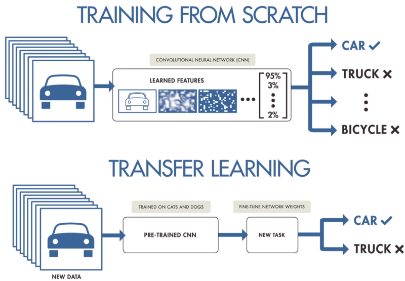
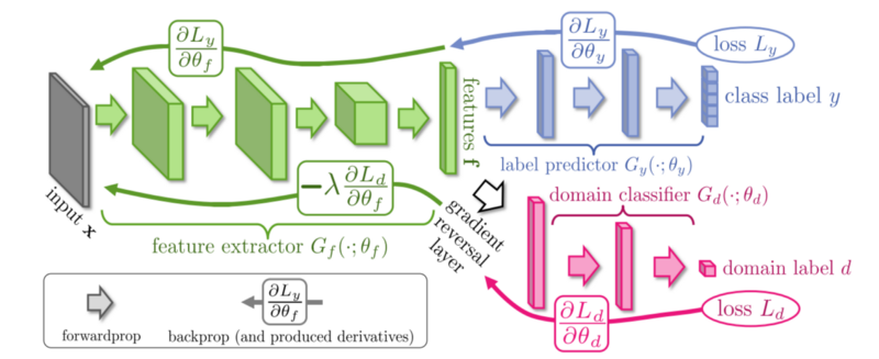
A Few images that tells you what Transfer learning is

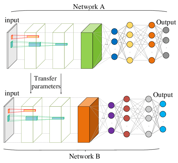
Several pre-trained models used in transfer learning are based on large convolutional neural networks (CNN).

With transfer learning, you use the early and middle layers and only re-train the latter layers.

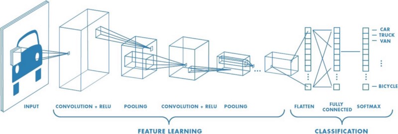
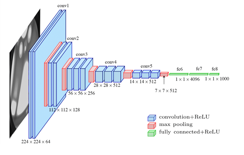
Typical CNN:

A Typical CNN consists of 2 important parts(look above figure):

1. Convolutional base/Feature learning(Conv+Relu+Pooling)
2. Classifier/Classification(Fully connected layer)
3. Convolutional base , which is composed by a stack of convolutional and pooling layers. The main goal of the convolutional base is to generate features from the image such as Edges/lines/curves in earlier layers and shapes in middle layers.
4. Classifier, which is usually composed by a fully connected layers. Classifier classifies the image based on the specific task related Features.

With transfer learning, you use the convolutional base and only re-train the classifier to your dataset.

Transfer learning scenarios:

Transfer learning can be used in 3 ways:

1. ConvNet as a fixed feature extractor/train as classifier
2. Finetuning the ConvNet/fine tune
3. Pretrained models

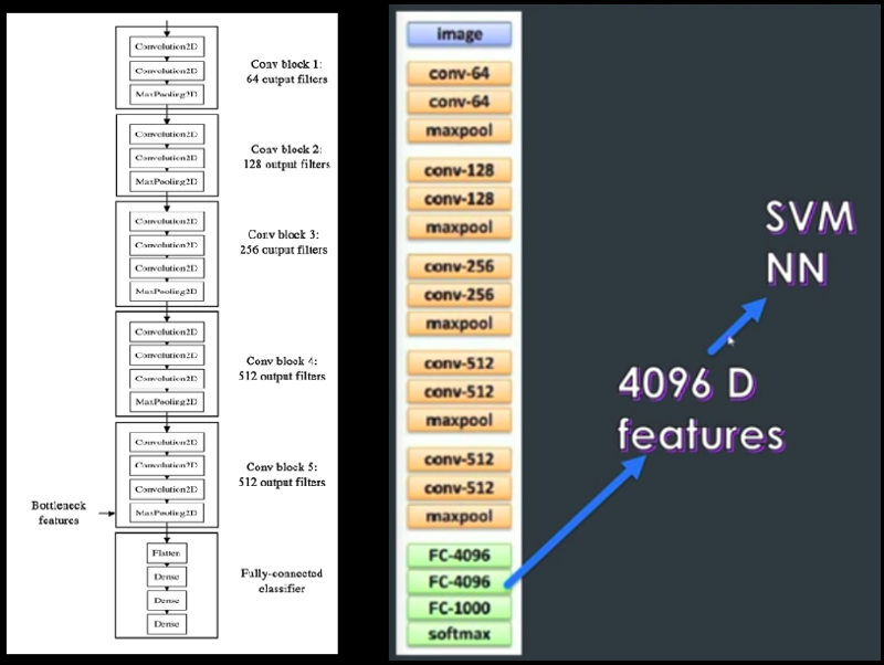
ConvNet as a fixed feature extractor:

Take a ConvNet(VGG-16) pretrained on ImageNet(1.2M input images,1000ouput class scores), then remove the last fully-connected layer (this layer’s outputs are the 1000 class scores for a different task like ImageNet), then treat the rest of the ConvNet as a fixed feature extractor for the new dataset.

In an VGG16 pretrained on ImageNet(below figure), this would compute a 4096-D vector for every image that contains the activations of the hidden layer immediately before the classifier. Once you extract the 4096-D codes for all images, train a linear classifier (e.g. Linear SVM or Softmax classifier) for the new dataset.

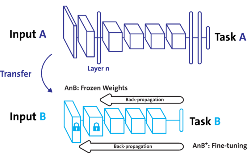
Finetuning the ConvNet:

The second strategy is to not only replace and retrain the classifier on top of the ConvNet on the new dataset, but to also fine-tune the weights of the pretrained network by continuing the backpropagation.

a) It is possible to fine-tune all the layers of the ConvNet, or b)it’s possible to keep some of the earlier layers fixed (due to overfitting concerns) and only fine-tune some higher-level portion of the network

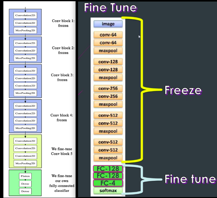
If you see this In left side image of VGG-16 the 1st 4 Conv blocks are frozen, last Conv and FC are tunned here, in right side image of VGG16 the 1st 5 Conv blocks are frozen , only last FC block was fine tunned here. its upto you and your datset to take of your choice.

Pretrained model:

Since modern ConvNets take 2–3 weeks to train across multiple GPUs on ImageNet, it is common to see people release their final ConvNet checkpoints for the benefit of others who can use the networks for fine-tuning.

How do you decide what type of transfer learning you should perform on a new dataset? This is a function of several factors, but the two most important ones are the size of the new dataset (small or big).

Transfer learning scenarios:

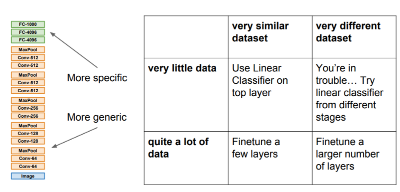
1. New dataset is small and similar to original dataset. Since the data is small, it is not a good idea to fine-tune the ConvNet due to overfitting concerns. Since the data is similar to the original data, we expect higher-level features in the ConvNet to be relevant to this dataset as well. Hence, the best idea might be to train a linear classifier on the CNN codes.
2. New dataset is large and similar to the original dataset. Since we have more data, we can have more confidence that we won’t overfit if we were to try to fine-tune through the full network.
3. New dataset is small but very different from the original dataset. Since the data is small, it is likely best to only train a linear classifier. Since the dataset is very different, it might not be best to train the classifier form the top of the network, which contains more dataset-specific features. Instead, it might work better to train the SVM classifier from activations somewhere earlier in the network.
4. New dataset is large and very different from the original dataset. Since the dataset is very large, we may expect that we can afford to train a ConvNet from scratch. However, in practice it is very often still beneficial to initialize with weights from a pretrained model. In this case, we would have enough data and confidence to fine-tune through the entire network.

Transfer learning using pytorch for image classification:

In this tutorial, you will learn how to train your network using transfer learning. I recommend to use google colab for fast computing and speeding up processing.

you can check out the entire code for google colab here in my github.

These two major transfer learning scenarios look as follows:

• Finetuning the convnet: Instead of random initializaion, we initialize the network with a pretrained network, like the one that is trained on imagenet 1000 dataset. Rest of the training looks as usual.
• ConvNet as fixed feature extractor: Here, we will freeze the weights for all of the network except that of the final fully connected layer. This last fully connected layer is replaced with a new one with random weights and only this layer is trained.

Packages:

from __future__ import print_function, division
import torch
import torch.nn as nn
import torch.optim as optim
from torch.optim import lr_scheduler
import numpy as np
import torchvision
from torchvision import datasets, models, transforms
import matplotlib.pyplot as plt
import time
import os
import copy
plt.ion()   # interactive mode

Data loading:

The training archive contains 25,000 images of dogs and cats. you can download and know more about the data here.

Data augmentation and normalization for training

Just normalization for validation

data_transforms = {
    'train': transforms.Compose([
        transforms.RandomResizedCrop(224),
        transforms.RandomHorizontalFlip(),
        transforms.ToTensor(),
        transforms.Normalize([0.485, 0.456, 0.406], [0.229, 0.224, 0.225])
    ]),
    'val': transforms.Compose([
        transforms.Resize(256),
        transforms.CenterCrop(224),
        transforms.ToTensor(),
        transforms.Normalize([0.485, 0.456, 0.406], [0.229, 0.224, 0.225])
    ]),
}
data_dir = '/content/Cat_Dog_data/'
image_datasets = {x: datasets.ImageFolder(os.path.join(data_dir, x),
                                          data_transforms[x])
                  for x in ['train','val']}
dataloaders = {x: torch.utils.data.DataLoader(image_datasets[x], batch_size=4,
                                             shuffle=True, num_workers=4)
              for x in ['train','val']}
dataset_sizes = {x: len(image_datasets[x]) for x in ['train','val']}
class_names = image_datasets['train'].classes
device = torch.device("cuda:0" if torch.cuda.is_available() else "cpu")

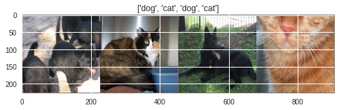
Visualize few images:

def imshow(inp, title=None):
    """Imshow for Tensor."""
    inp = inp.numpy().transpose((1, 2, 0))
    mean = np.array([0.485, 0.456, 0.406])
    std = np.array([0.229, 0.224, 0.225])
    inp = std * inp + mean
    inp = np.clip(inp, 0, 1)
    plt.imshow(inp)
    if title is not None:
        plt.title(title)
    plt.pause(0.001)  # pause a bit so that plots are updated
# Get a batch of training data
inputs, classes = next(iter(dataloaders['train']))
# Make a grid from batch
out = torchvision.utils.make_grid(inputs)
imshow(out, title=[class_names[x] for x in classes])

Training the model

Now, let’s write a general function to train a model. Here, we will illustrate:

• Scheduling the learning rate
• Saving the best model

In the following, parameter scheduler is an LR scheduler object from torch.optim.lr_scheduler.

def train_model(model, criterion, optimizer, scheduler, num_epochs=25):
    since = time.time()
    best_model_wts = copy.deepcopy(model.state_dict())
    best_acc = 0.0
    for epoch in range(num_epochs):
        print('Epoch {}/{}'.format(epoch, num_epochs - 1))
        print('-' * 10)
        # Each epoch has a training and validation phase
        for phase in ['train', 'val']:
            if phase == 'train':
                scheduler.step()
                model.train()  # Set model to training mode
            else:
                model.eval()   # Set model to evaluate mode
            running_loss = 0.0
            running_corrects = 0
            # Iterate over data.
            for inputs, labels in dataloaders[phase]:
                inputs = inputs.to(device)
                labels = labels.to(device)
                # zero the parameter gradients
                optimizer.zero_grad()
                # forward
                # track history if only in train
                with torch.set_grad_enabled(phase == 'train'):
                    outputs = model(inputs)
                    _, preds = torch.max(outputs, 1)
                    loss = criterion(outputs, labels)
                    # backward + optimize only if in training phase
                    if phase == 'train':
                        loss.backward()
                        optimizer.step()
                # statistics
                running_loss += loss.item() * inputs.size(0)
                running_corrects += torch.sum(preds == labels.data)
            epoch_loss = running_loss / dataset_sizes[phase]
            epoch_acc = running_corrects.double() / dataset_sizes[phase]
            print('{} Loss: {:.4f} Acc: {:.4f}'.format(
                phase, epoch_loss, epoch_acc))
            # deep copy the model
            if phase == 'val' and epoch_acc > best_acc:
                best_acc = epoch_acc
                best_model_wts = copy.deepcopy(model.state_dict())
        print()
    time_elapsed = time.time() - since
    print('Training complete in {:.0f}m {:.0f}s'.format(
        time_elapsed // 60, time_elapsed % 60))
    print('Best val Acc: {:4f}'.format(best_acc))
    # load best model weights
    model.load_state_dict(best_model_wts)
    return model

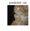
Visualizing the model predictions:

Generic function to display predictions for a few images

def visualize_model(model, num_images=6):
    was_training = model.training
    model.eval()
    images_so_far = 0
    fig = plt.figure()
    with torch.no_grad():
        for i, (inputs, labels) in enumerate(dataloaders['val']):
            inputs = inputs.to(device)
            labels = labels.to(device)
            outputs = model(inputs)
            _, preds = torch.max(outputs, 1)
            for j in range(inputs.size()[0]):
                images_so_far += 1
                ax = plt.subplot(num_images//2, 2, images_so_far)
                ax.axis('off')
                ax.set_title('predicted: {}'.format(class_names[preds[j]]))
                imshow(inputs.cpu().data[j])
                if images_so_far == num_images:
                    model.train(mode=was_training)
                    return
        model.train(mode=was_training)

Finetuning the convnet:

Load a pretrained model and reset final fully connected layer.

model_ft = models.resnet18(pretrained=True)
num_ftrs = model_ft.fc.in_features
model_ft.fc = nn.Linear(num_ftrs, 2)
model_ft = model_ft.to(device)
criterion = nn.CrossEntropyLoss()
# Observe that all parameters are being optimized
optimizer_ft = optim.SGD(model_ft.parameters(), lr=0.001, momentum=0.9)
# Decay LR by a factor of 0.1 every 7 epochs
exp_lr_scheduler = lr_scheduler.StepLR(optimizer_ft, step_size=7, gamma=0.1)

Train and evaluate

It should take around 45–60 min on CPU. On GPU though, it takes less than a hour as we are working on dataset of huge size of 25000 images.

model_ft = train_model(model_ft, criterion, optimizer_ft, exp_lr_scheduler,num_epochs=25)

at last epoch:

Epoch 24/24
----------
train Loss: 0.0822 Acc: 0.9650
val Loss: 0.0315 Acc: 0.9876
Training complete in 133m 50s
Best val Acc: 0.988400

We got the Accuracy on validation set of 98.84%

Visualise the output

visualize_model(model_ft)

Similar tutorial

You can find similar tutorial on Ants and Bees here in the official pytorch website here.

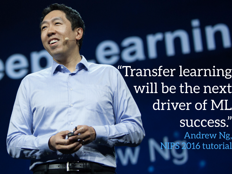
Great minds on transfer learning:

Summary:

• Transfer learning

• Pretrained model

• A Typical CNN

1. Convolutional base
2. Classifier

• Transfer learning scenarios:

1. ConvNet as a fixed feature extractor/train as classifier
2. Finetuning the ConvNet/fine tune
3. Pretrained models

• Transfer learning using pytorch for image classification

Programme/code/application of transfer learning above in this blog with 98% accuracy

References/some other great tutorials:

Sebastian Ruder blog.

Andrej karpathy blog.

Hacker earth blog.

Pytorch Transfer learning blog.