Recurrent neural networks and lstm explained
Published:
In this post we are going to explore RNN’s and LSTM’s.
you can chek out this blog on my medium page here
Recurrent Neural Networks are the first of its kind State of the Art algorithms that can Memorize/remember previous inputs in memory, When a huge set of Sequential data is given to it.
Before we dig into details of Recurrent Neural networks, if you are a Beginner i suggest you to read A Beginner intro to Neural Networks and A Beginner intro to Convolutional Neural Networks.
Now in this, we will learn:
- what are Neural Networks?
- what Neural Networks do?
- why not Neural Networks/Feed forward Networks?
- Why/what are Recurrent Neural Networks?
- Different Types of RNN’s
- Deep view into RNN’s
- Character level language model
- Back propogation through time(BTT)
- Issues of RNN’s?
- Advantages & Disadvantages of RNN
- Why LSTM’s?
- Forget gate
- input gate
- output gate.
- Resources
What are Neural networks?
Neural networks are set of algorithms inspired by the functioning of human brian. Generally when you open your eyes, what you see is called data and is processed by the Nuerons(data processing cells) in your brain, and recognises what is around you. That’s how similar the Neural Networks works. They takes a large set of data, process the data(draws out the patterns from data), and outputs what it is.
What they do ?
Neural networks sometimes called as Artificial Neural networks(ANN’s), because they are not natural like neurons in your brain. They artifically mimic the nature and funtioning of Neural network. ANN’s are composed of a large number of highly interconnected processing elements (neurones) working in unison to solve specific problems.
ANNs, like people,like child, they even learn by example. An ANN is configured for a specific application, such as pattern recognition or data classification,Image recognition, voice recognition through a learning process.
Neural networks (NN) are universal function approximaters so that means neural networks can learn an approximation of any function f() such that.
y = f(x)
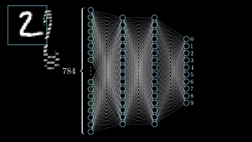
NN trying to predict the image(data) that given to it. it predicts that the no is 2 here
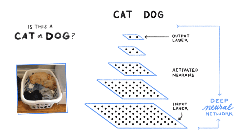 A Neural network/feed forward Neural network predicting cat image.
you can read more about Artificial Neural Networks here.
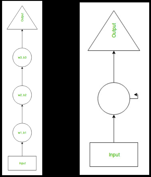
Why Not Neural Networks/Feed forward Networks?
A trained Feed Forward Neural Network can be Exposed to any huge random collection of images and asked to predict the output. for example check out the below figure
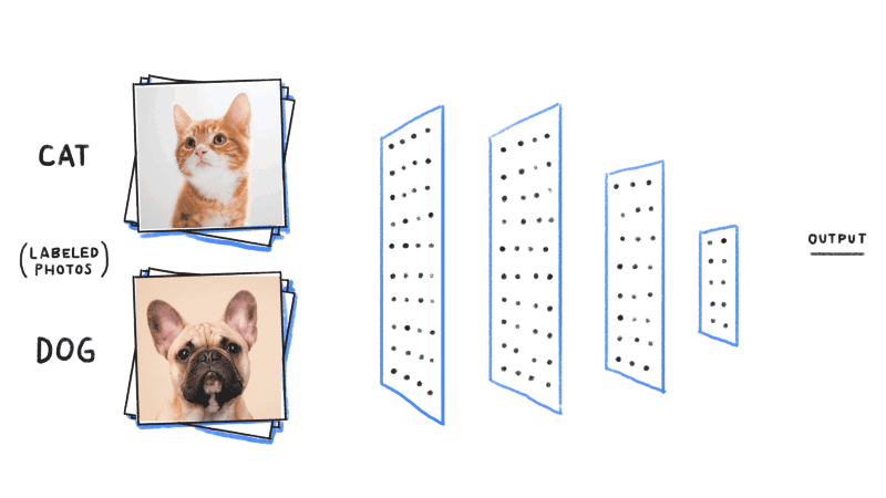
In this training process, the first picture that the Neural network exposed to, will not necessarly alter how it classifies the Second one.
here the output of Cat does not relate to the output Dog. There are several scenario’s where the previous understanding of data is important.for example: Reading book, understanding lyrics,..,. These networks do not have memory in order to understand Sequential data like Reading books.
how do we overcome this challenge of understanding previous output?
solution: RNN’s.
What are RNN’s?
The idea behind RNNs is to make use of sequential information. In a traditional neural network we assume that all inputs (and outputs) are independent of each other. But for many tasks that’s a very bad idea. If you want to predict the next word in a sentence you better know which words came before it. RNNs are called recurrent because they perform the same task for every element of a sequence, with the output being depended on the previous computations and you already know that they have a “memory” which captures information about what has been calculated so far.
“Whenever there is a sequence of data and that temporal dynamics that connects the data is more important than the spatial content of each individual frame.” – Lex Fridman (MIT)
More about RNN’s explained below.
Different types of RNN’s
The core reason that recurrent nets are more exciting is that they allow us to operate over sequences of vectors: Sequences in the input, the output, or in the most general case both. A few examples may make this more concrete:
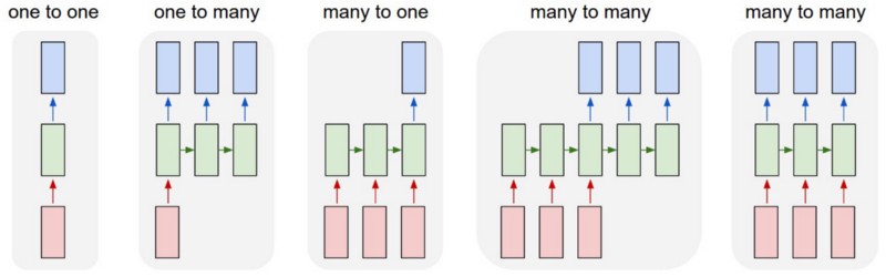
Each rectangle in above image represent Vectors and Arrows represent functions. Input vectors are Red in color, output vectors are blue and green holds RNN’s state.
One-to-one:
This also called as Plain/Vaniall Neural networks. It deals with Fixed size of input to Fixed size of Output where they are independent of previous information/output.
Ex: Image classification.
One-to-Many:
it deals with fixed size of information as input that gives sequence of data as output.
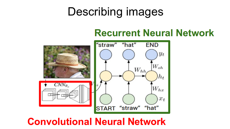
Ex: Image Captioning takes image as input and outputs a sentence of words.
Many-to-One:
It takes Sequence of information as input and ouputs a fixed size of output.
Ex: sentiment analysis where a given sentence is classified as expressing positive or negative sentiment.
Many-to-Many:
It takes a Sequence of information as input and process it recurrently outputs a Sequence of data.
Ex: Machine Translation, where an RNN reads a sentence in English and then outputs a sentence in French.
Bidirectional Many-to-Many:
Synced sequence input and output. Notice that in every case are no pre-specified constraints on the lengths sequences because the recurrent transformation (green) is fixed and can be applied as many times as we like.
Ex: video classification where we wish to label each frame of the video.
CNN vs RNN:
I dont think you need explanation for this. You can easily get what it is just by looking at the figure below:
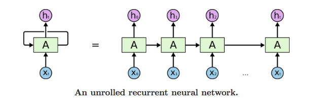
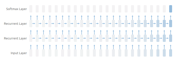
Deep view into RNN’s:
In a simple Neural Network you can see Input unit, hidden units and output units that process information independently having no relation to previous one. Also here we gave different weights and bias to the hidden units giving no chance to memorize any information.
where Hidden layer in RNN’s have same weights and bias through out the process giving them the chance to memorize information processed through them.
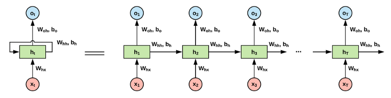 Current time stamp:
look at the above figure, where the formula for the Current state:
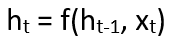
where Ot is output state, ht →current time stamp, ht-1 → is previous time stamp, and xt is passed as input state.
Applying activation function:
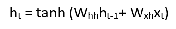
W is weight, h is the single hidden vector, Whh is the weight at previous hidden state, Whx is the weight at current input state.
Where tanh is the Activation funtion, that implements a Non-linearity that squashes the activations to the range[-1.1]
Output:
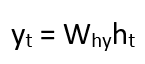
Yt is the output state. Why is the weight at the output state.
Example: “Character level language model” explained below.
Character level language model:
We’ll give the RNN a huge chunk of text and ask it to model the probability distribution of the next character in the sequence given a sequence of previous characters.
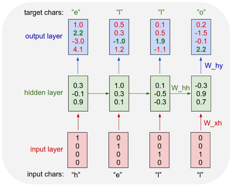
As a working example, suppose we only had a vocabulary of four possible letters “helo”, and wanted to train an RNN on the training sequence “hello”. This training sequence is in fact a source of 4 separate training examples: 1. The probability of “e” should be likely given the context of “h”, 2. “l” should be likely in the context of “he”, 3. “l” should also be likely given the context of “hel”, and finally 4. “o” should be likely given the context of “hell”.
you can get more about this example here and here.
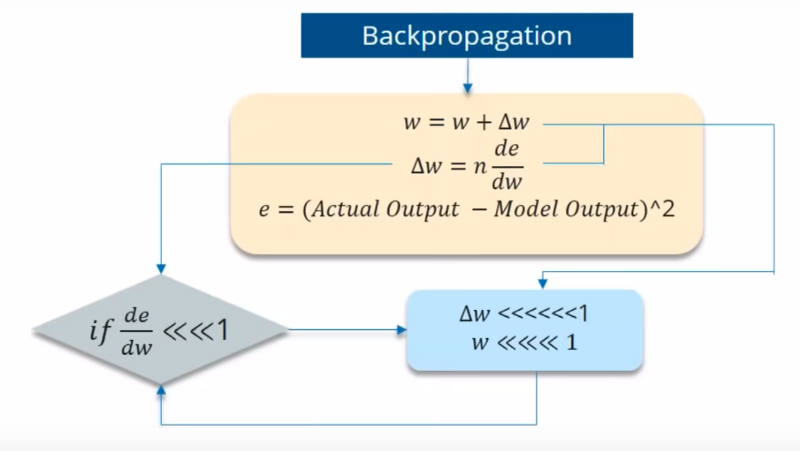
Backpropogate Through Time:
To understand and visualize the Backpropogation, lets unroll the network at all the time stamps, so that you can see how the weights gets updated.Going back in Every time stamp to change/update the weights is called Backpropogate through time.
 We typically treat the full sequence (word) as one training example, so the total error is just the sum of the errors at each time step (character). The weights as we can see are the same at each time step. Let’s summarize the steps for backpropagation through time
The cross entropy error is first computed using the current output and the actual output.
Remember that the network is unrolled for all the time steps.
For the unrolled network, the gradient is calculated for each time step with respect to the weight parameter.
Now that the weight is the same for all the time steps the gradients can be combined together for all time steps.
The weights are then updated for both recurrent neuron and the dense layers.
Note: Going back into every time stamp and updating its weights is really a slow process. It takes both the computational power and time.
While Backpropogating you may get 2 types of issues.
- Vanishing Gradient
- Exploding Gradient
Vanishing Gradient:
where the contribution from the earlier steps becomes insignificant in the gradient descent step.
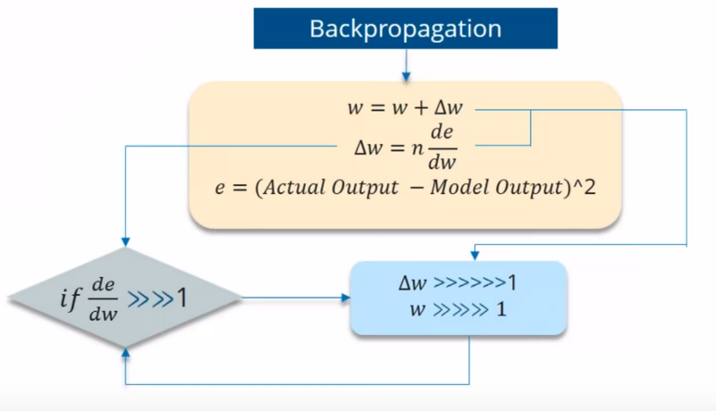
While you are using Backpropogating through time, you find Error is the difference of Actual and Predicted model. Now what if the partial derivation of error with respect to weight is very less than 1?
If the partial derivation of Error is less than 1, then when it get multiplied with the Learning rate which is also very less. then Multiplying learning rate with partial derivation of Error wont be a big change when compared with previous iteration.
For ex:- Lets say the value decreased like 0.863 →0.532 →0.356 →0.192 →0.117 →0.086 →0.023 →0.019..
you can see that there is no much change in last 3 iterations. This Vanishing of Gradience is called Vanishing Gradience.
Aslo this Vanishing gradient problem results in long-term dependencies being ignored during training.
you Can Visualize this Vanishing gradient problem at real time here.
Several solutions to the vanishing gradient problem have been proposed over the years. The most popular are the aforementioned LSTM and GRU units, but this is still an area of active research.
Exploding Gradient:
We speak of Exploding Gradients when the algorithm assigns a stupidly high importance to the weights, without much reason. But fortunately, this problem can be easily solved if you truncate or squash the gradients.
similarly here, What if the Partial derivation of Errror is more than 1? Think.
How can you overcome the Challenges of Vanishing and Exploding Gradience?
- Vanishing Gradience can be overcome with
- Relu activation function.
- LSTM, GRU.
- Exploding Gradience can be overcome with
- Truncated BTT(instead starting backprop at the last time stamp, we can choose similar time stamp, which is just before it.)
- Clip Gradience to threshold.
- RMSprop to adjust learning rate.
Advantages of Recurrent Neural Network
- The main advantage of RNN over ANN is that RNN can model sequence of data (i.e. time series) so that each sample can be assumed to be dependent on previous ones
- Recurrent neural network are even used with convolutional layers to extend the effective pixel neighborhood.
Disadvantages of Recurrent Neural Network
- Gradient vanishing and exploding problems.
- Training an RNN is a very difficult task.
- It cannot process very long sequences if using tanh or relu as an activation function.
Long Short Term Memory:
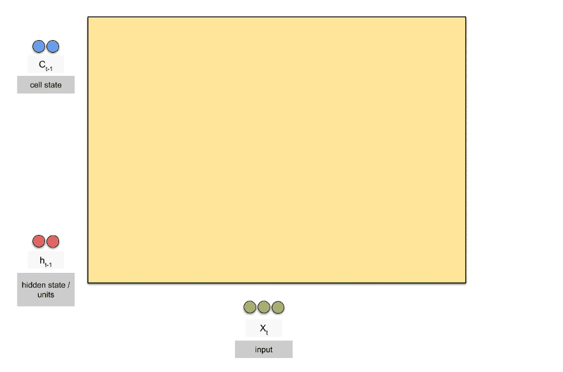
A special kind of RNN’s, capable of Learning Long-term dependencies.
LSTM’s have a Nature of Remembering information for a long periods of time is their Default behaviour.
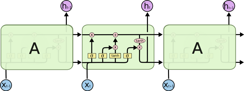
LSTM had a three step Process:
look at the below figure that says Every LSTM module will have 3 gates named as Forget gate, Input gate, Output gate.
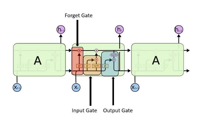
Forget Gate:
Decides how much of the past you should remember.
This gate Decides which information to be omitted in from the cell in that particular time stamp. It is decided by the sigmoid function. it looks at the previous state(ht-1) and the content input(Xt) and outputs a number between 0(omit this)and 1(keep this)for each number in the cell state Ct−1.
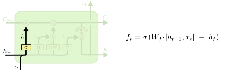
EX: lets say ht-1 →Roufa and Manoj plays well in basket ball.
Xt →Manoj is really good at webdesigning.
- Forget gate realizes that there might be change in the context after encounter its first fullstop.
- Compare with Current Input Xt.
- Its important to know that next sentence, talks about Manoj. so information about Roufa is omited.
Update Gate/input gate:
Decides how much of this unit is added to the current state.
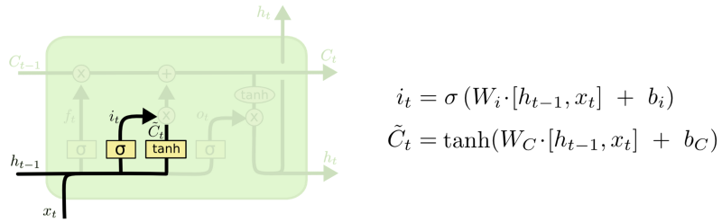
Sigmoid function decides which values to let through 0,1. and tanh function gives weightage to the values which are passed deciding their level of importance ranging from -1 to 1.
EX: Manoj good webdesigining, yesterday he told me that he is a university topper.
input gate analysis the important information.
Manoj good webdesigining, he is university topper is important.
yesterday he told me that is not important, hence forgotten.
Output Gate:
Decides which part of the current cell makes it to the output.
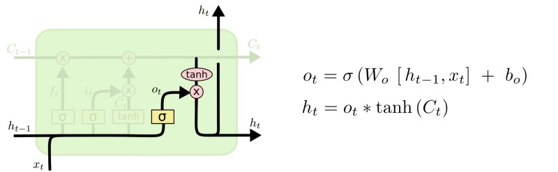
Sigmoid function decides which values to let through 0,1. and tanh function gives weightage to the values which are passed deciding their level of importance ranging from -1 to 1 and multiplied with output of Sigmoid.
EX: Manoj good webdesigining, he is university topper so the Merit student _______ was awarded University Gold medalist.
- there could be lot of choices for the empty dash. this final gate replaces it with Manoj.
A Blog on LSTM’s with Nice visualization is here.
Resources:
checkout resources at my medium blog here.
Thank you
Thank you so much for landing on this page.