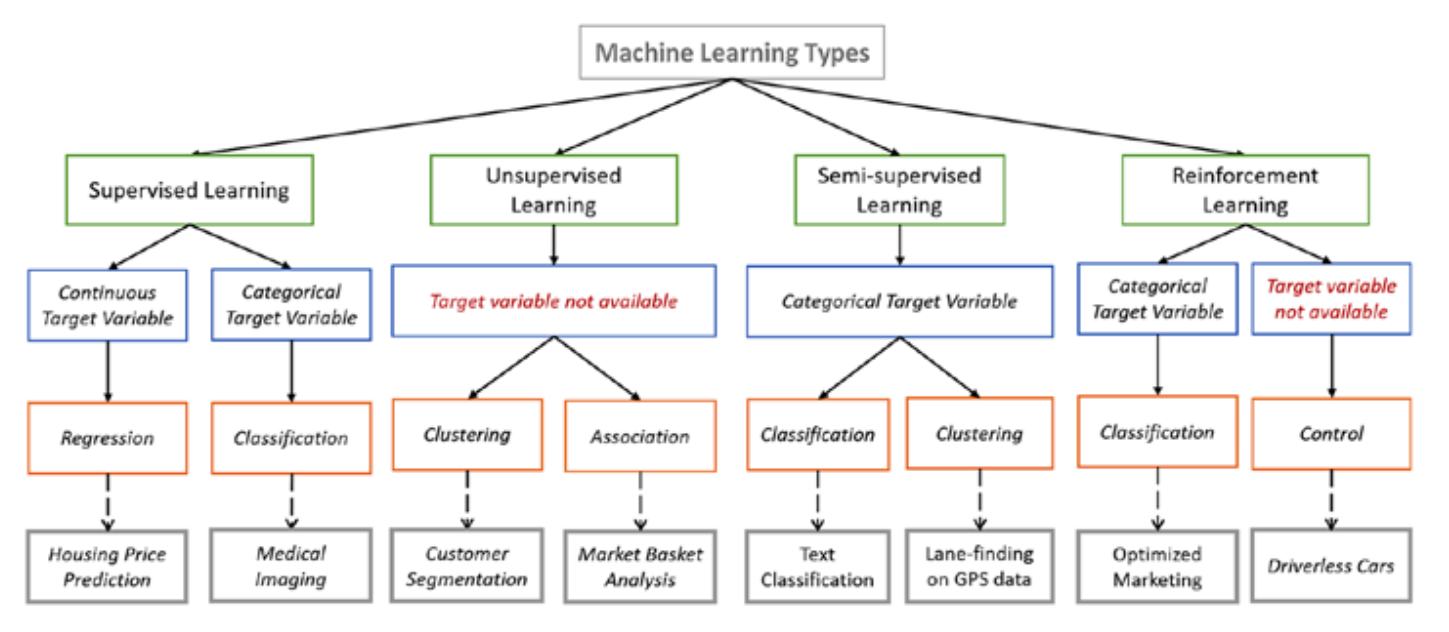
Machine learning has Several algorithms like

1. Linear regression
2. Logistic regression
3. k-Nearest neighbors
4. k- Means clustering
5. Support Vector Machines
6. Decision trees
7. Random Forest
8. Gaussian Naive Bayes

Today we will look in to Linear regression algorithm.

Linear Regression:

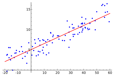
Linear regression is most simple and every beginner Data scientist or Machine learning Engineer start with this. Linear regression comes under supervised model where data is labelled. In linear regression we will find relationship between one or more features(independent variables) like x1,x2,x3………xn. and one continuous target variable(dependent variable) like y.

The thing is to find the relationship/best fit line between 2 variables. if it is just between the 2 variables then it is callled Simple LinearRegression. if it is between more than 1 variable and 1 target variable it is called Multiple linearregression.

Equation:

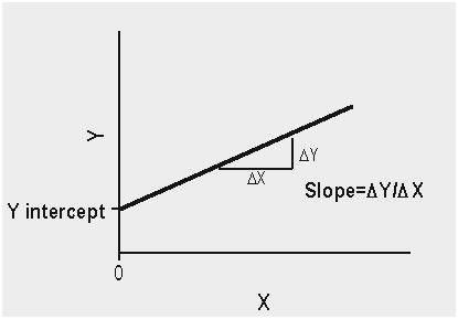
1. for simple linear regression it is just

y = mx+c , with different notation it is

y =wx +b.

where y = predicted,dependent,target variable. x = input,independent,actual

m(or)w = slope, c(or)b = bias/intercept.

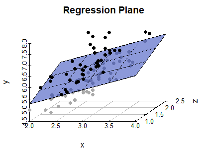
1. for mulitple linear regression it is just the sum of all the variables which is summation of variables like x1,x2,x3………xn,with weights w1,w2,w3…wn. to variable y.

y = w1.x1 + w2.x2 + w3.x3…………wn.xn + c

with summation it is

y= summation(wi.xi)+c, where i goes from 1,2,3,4……….n

m = slope, which is Rise(y2-y1)/Run(x2-x1).

you can find slope between 2 points a=(x1,y1) b=(x2,y2). allocate some points and tryout yourself.

Realtime examples:

1. predicting height of a person with respect to weight from Existing data.
2. predicting the rainfall in next year from the historical data.
3. Monthly spending amount for your next year.
4. no.of. hours studied vs marks obtained as i said earlier our goal is to get the best fit line to the given data.

But how do we get the Best fit line?

yes, its by decreasing the cost function.

But, how do we find the cost funtion?

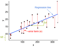
Cost function:

a cost function is a measure of how wrong the model is in terms of its ability to estimate the relationship between X and y.

here are 3 error functions out of many:

1. MSE(Mean Squared Error)
2. RMSE(Root Mean Squared Error)
3. Logloss(Cross Entorpy loss) people mostly go with MSE.

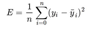which is nothing but

Where y1,y2,y3 are actual values and y’1,y’2,y’3 are predicted values.

now you got the Cost Function which means you got Error values. all you have to do now is to decrease the Error which means decrease the cost function.

But how do we Decrese the cost function?

By using Gradient Descent.

Gradient Descent:

We apply Derivation function on Cost function, so that the Error reduces.

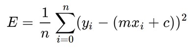
1. Take the cost function is

1. after applying Partial derivative with respect to “m” and “b” , it looks like this

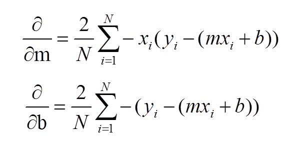
1. now add some learning rate “alpha” to it.

note: do not get confused with notations. just write down equations on paper step by step, so that you wont get confused. 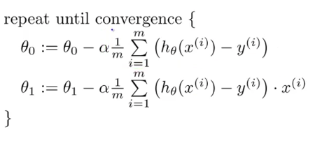“theta0” is “b” in our case,

“theta1” is “m” in our case which is nothing but slope

‘m” is “N” in our case

and ‘alpha’ is learning rate. 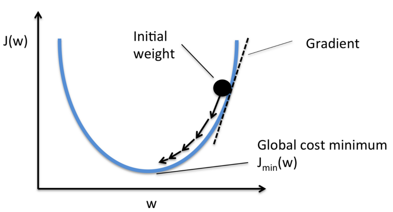in 3d it looks like 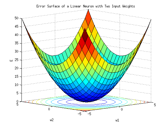“alpha value” (or) ‘alpha rate’ should be slow. if it is more leads to “overfit”, if it is less leads to “underfit”. 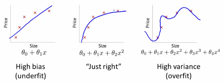still if you dont get what Gradient Descent is have a look at some youtube videos. Done.

For simple understanding all you need to remember is just 4 steps:

1. goal is to find the best fit for all our data points so that our predictions are much accurate.
2. To get the best fit, we must reduce the Error, cost function comes into play here.
3. cost function finds error.
4. Gradient descent reduces error with “derivative funcion” and “alpharate”. Now the interesting part comes. its coding.

CODE

`# importing libraries #for versions checkout requirements.txt import numpy as np import pandas as pd import matplotlib.pyplot as plt #importing and reading data sets data = pd.read_csv(“bmi_and_life.csv”) #look at top 5 rows in data set data.head() #delete/drop ‘Country’ variable. data = data.drop([‘Country’], axis = 1) #reading into variables X = data.iloc[:, :-1].values Y = data.iloc[:, 1].values from sklearn.model_selection import train_test_split X_train,X_test,y_train,y_test = train_test_split(X,Y, test_size = 20, random_state = 0) #import linear regression from sklearn.linear_model import LinearRegression lr = LinearRegression() #fitting the model lr.fit(X_train,y_train) LinearRegression(copy_X=True, fit_intercept=True, n_jobs=1, normalize=False)

Predicting the Test set results

y_pred = lr.predict(X_test)`

For visualization and for more explanation check out the github repo here

Thank you.

Thank you for landing on this page.

References:

1. https://spin.atomicobject.com/2014/06/24/gradient-descent-linear-regression/
2. https://blog.algorithmia.com/introduction-to-loss-functions/
3. https://www.kdnuggets.com/2018/10/linear-regression-wild.html