A beginner intro to neural networks

you are going to explore Neural Networks

checkout this blog on my medium page here

What are Neural networks?

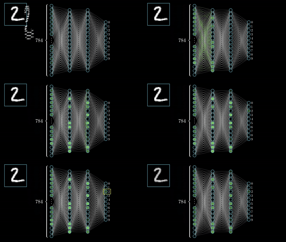
Neural networks are set of algorithms inspired by the functioning of human brian. Generally when you open your eyes, what you see is called data and is processed by the Nuerons(data processing cells) in your brain, and recognises what is around you. That’s how similar the Neural Networks works. They takes a large set of data, process the data(draws out the patterns from data), and outputs what it is.

What they do ?

Neural networks sometimes called as Artificial Neural networks(ANN’s), because they are not natural like neurons in your brain. They artifically mimic the nature and funtioning of Neural network. ANN’s are composed of a large number of highly interconnected processing elements (neurones) working in unison to solve specific problems.

ANNs, like people,like child, they even learn by example. An ANN is configured for a specific application, such as pattern recognition or data classification,Image recognition, voice recognition through a learning process.

Neural networks (NN) are universal function approximaters so that means neural networks can learn an approximation of any function f() such that.

y = f(x)

you can check several other Neural Networks here.

Why use Neural networks?

Neural networks, with their remarkable ability to derive meaning from complicated or imprecise data, can be used to extract patterns and detect trends that are too complex to be noticed by either humans or other computer techniques. A trained neural network can be thought of as an “expert” in the category of information it has been given to analyse. This expert can then be used to provide projections given new situations of interest and answer “what if” questions. Other advantages include:

1. Adaptive learning: An ability to learn how to do tasks based on the data given for training or initial experience.
2. Self-Organisation: An ANN can create its own organisation or representation of the information it receives during learning time.

Network layers

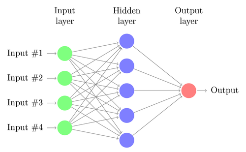
The commonest type of artificial neural network consists of three groups, or layers, of units: a layer of “input” units is connected to a layer of “hidden” units, which is connected to a layer of “output” units. (see Figure 4.1)

• Input units:- The activity of the input units represents the raw information that is fed into the network. this also called input layer.

• Hidden units:- The activity of each hidden unit is determined by the activities of the input units and the weights on the connections between the input and the hidden units. this also called hidden layer.

• Output units:- The behaviour of the output units depends on the activity of the hidden units and the weights between the hidden and output units. this also called output layer. Nueral Network with Input layer, Hiddenlayer, Output layer

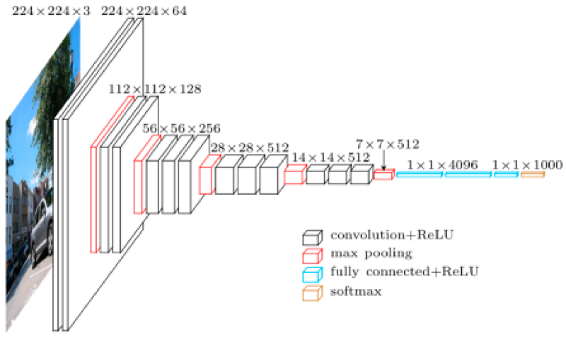
you can check several other Neural networks and their layers here. so that you will come to know how they looks.

This simple type of network is interesting because the hidden units are free to construct their own representations of the input. The weights between the input and hidden units determine when each hidden unit is active, and so by modifying these weights, a hidden unit can choose what it represents.

Before we look into entire/Deep Neural Network lets look into a single neuron.

A Single Neuron

The basic unit of computation in a neural network is the neuron, often called as a node or unit. It receives input from some other nodes, or from an external source and computes an output. Each input has an associated weight (w), which is assigned on the basis of its relative importance to other inputs. The node applies a function f (defined below) to the weighted sum of its inputs as in figure below.

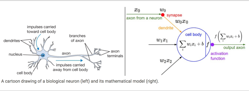
The above network takes numerical inputs X1 and X2 and has weights w1 and w2 associated with those inputs. Additionally, there is another input 1 with weight b (called the Bias) associated with it.

Activation function:

The output Y from the neuron is computed as shown in the Figure above. The function f is non-linear and is called the Activation Function. The purpose of the activation function is to introduce non-linearity into the output of a neuron. This is important because most real world data is non linear and we want neurons to learn these non linear representations.

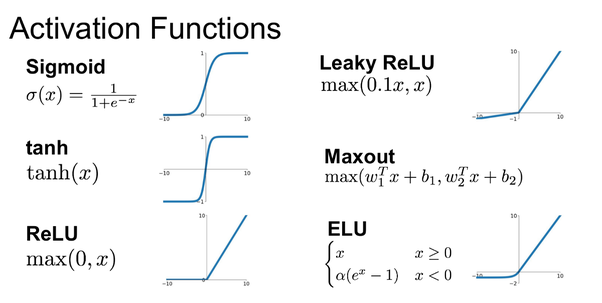
Every activation function (or non-linearity) takes a single number and performs a certain fixed mathematical operation on it. There are several activation functions you may encounter in practice:

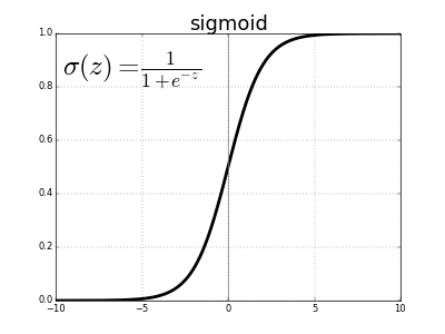
• Sigmoid: takes a real-valued input and squashes it to range between 0 and 1

σ(x) = 1 / (1 + exp(−x))

• Softmax function: In classification tasks, we generally use a Softmax function as the Activation Function in the Output layer of the Multi Layer Perceptron to ensure that the outputs are probabilities and they add up to 1. The Softmax function takes a vector of arbitrary real-valued scores and squashes it to a vector of values between zero and one that sum to one. So, in this case,

Probability (Pass) + Probability (Fail) = 1

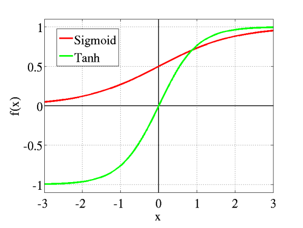
• tanh: takes a real-valued input and squashes it to the range [-1, 1]

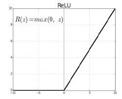
• ReLU: ReLU stands for Rectified Linear Unit. It takes a real-valued input and thresholds it at zero (replaces negative values with zero) f(x) = max(0, x)

The below figures shows several other activation functions.

Importance of Bias: The main function of Bias is to provide every node with a trainable constant value (in addition to the normal inputs that the node receives). See this link to learn more about the role of bias in a neuron.

Every Neural Network has 2 main parts:

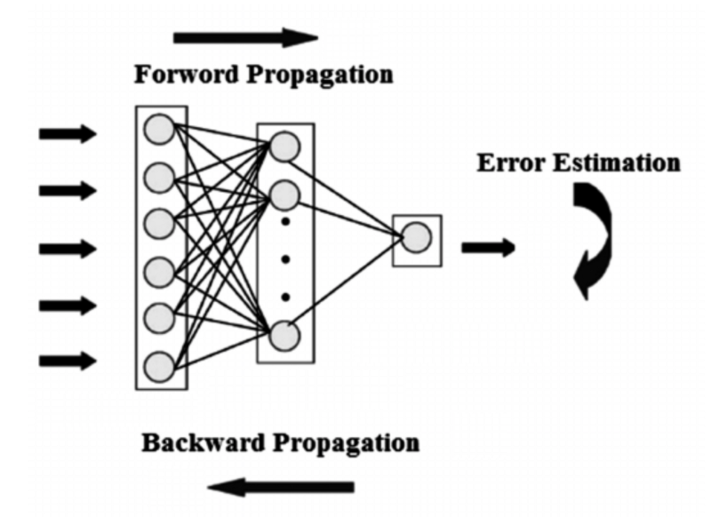
1. Feed Forward Propogation/Forward Propogation.
2. Backward Propogation/Back propogation. lets look at each individual parts.

Feed Forward Propogation:

All weights in the network are randomly assigned. Assume the weights of the connections from the inputs to that node are w1, w2 and w3.

The network then takes the first training example as input (we know that for inputs 35 and 67, the probability of Pass is 1).

• Input to the network = [35, 67]
• Desired output from the network (target) = [1, 0]

Then output V from the node in consideration can be calculated as below (f is an activation function such as sigmoid):

V = f (1w1 + 35w2 + 67*w3)

Similarly, outputs from the other node in the hidden layer is also calculated. The outputs of the two nodes in the hidden layer act as inputs to the two nodes in the output layer. This enables us to calculate output probabilities from the two nodes in output layer.

Suppose the output probabilities from the two nodes in the output layer are 0.4 and 0.6 respectively (since the weights are randomly assigned, outputs will also be random). We can see that the calculated probabilities (0.4 and 0.6) are very far from the desired probabilities (1 and 0 respectively), hence the network in Figure 5 is said to have an ‘Incorrect Output’.

Back Propagation and Weight Updation:

We calculate the total error at the output nodes and propagate these errors back through the network using Backpropagation to calculate the gradients. Then we use an optimization method such as Gradient Descent to ‘adjust’ all weights in the network with an aim of reducing the error at the output layer.

Suppose that the new weights associated with the node in consideration are w4, w5 and w6 (after Backpropagation and adjusting weights).

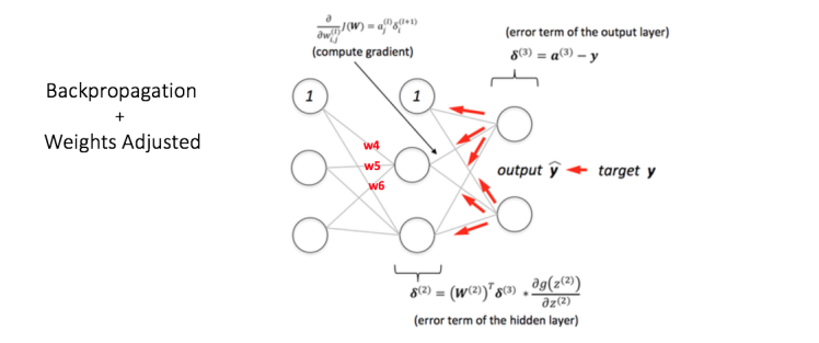
If we now input the same example to the network again, the network should perform better than before since the weights have now been adjusted to minimize the error in prediction. As shown in Figure 7, the errors at the output nodes now reduce to [0.2, -0.2] as compared to [0.6, -0.4] earlier. This means that our network has learnt to correctly classify our first training example.

We repeat this process with all other training examples in our dataset. Then, our network is said to have learnt those examples.

If we now want to predict whether a student studying 25 hours and having 70 marks in the mid term will pass the final term, we go through the forward propagation step and find the output probabilities for Pass and Fail.

I have avoided mathematical equations and explanation of concepts such as ‘Gradient Descent’ here and have rather tried to develop an intuition for the algorithm. For a more mathematically involved discussion of the Backpropagation algorithm, refer to this link.

Check out the Beginner intro to Convolution Neural Networks here.

References:

Feed forward and Backprop are reproduced from here.

Analytics vidhya blog here.

Skymind blog here.

Thank you

Thank you for being here